Chapter 9 Big data

9.1 The Big Picture

Big data problem: data is too big to fit into memory (=local environment).
R reads data into random-access memory (RAM) at once, and this object lives in memory entirely. So, if object.size > memory.size, the process will crash R.
Therefore, the key to dealing with big data in R is reducing the size of data you want to bring into it.

Techniques to deal with big data

Medium-sized file (1-2 GB)
- Try to reduce the size of the file using slicing and dicing
- Tools:
  - R:data.table::fread(file path, select = c("column 1", "column 2")). This command imports data faster than read.csv() does.
  - Command-line: csvkit - a suite of command-line tools to and working with CSV
Large file (> 2-10 GB)
- Put the data into a database and ACCESS it
- Explore the data and pull the objects of interest

Databases

Types of databases
- Relational database = a collection of tables (fixed columns and rows): SQL is a staple tool to define, query (the focus of the workshop today), control, and manipulate this type of database
- Non-relational database = a collection of documents (MongoDB), key-values (Redis and DyanoDB), wide-column stores (Cassandra and HBase), or graph (Neo4j and JanusGraph). Note that this type of database does not preclude SQL. NoSQL stands for “not only SQL.”

Relational database example

Relational Database. Source: MySQL Tutorial

9.2 SQL

Structured Query Language. Called SEQUEL and was developed by IBM Corporation in the 1970s.
Remains the standard language for a relational database management system.
It’s a DECLARATIVE language (what to do > how to do)
- Database management systems figure an optimal way to execute a query (query optimization)

SELECT COLUMN FROM TABLE

9.2.1 Learning objectives

Embracing a new mindset: shifting from ownership (opening CSVs stored in your laptop) to access (accessing data stored in a database)
Learning how to use R and SQL to access and query a database

9.2.2 SQL and R

SQL and R

SQL	R
SELECT	select() for columns, mutate() for expressions, summarise() for aggregates
FROM	which data frame
WHERE	filter()
GROUP BY	group_by()
HAVING	filter() after group_by()
ORDER BY	arrange()
LIMIT	head()

Challenge 1

Can you tell me the difference in the order in which the following R and SQL codes were written to manipulate data? For instance, in R, what command comes first? In contrast, in SQL, what command comes first?

R example


data %>% # Data 
  select() %>% # Column
  filter() %>% # Row 
  group_by() %>% # Group by 
  summarise(n = n()) %>% # n() is one of the aggregate functions in r; it's count() used inside summarise() function 
  filter() %>% # Row 
  order_by() # Arrange

SQL example (in a SQL chunk, use -- instead of # to comment)


SELECT column, aggregation (count())` -- Column

FROM data # Data 

WHERE condition -- Filter rows 

GROUP BY column -- Group by

HAVING condition -- Filter rows after group by  

ORDER BY column -- Arrange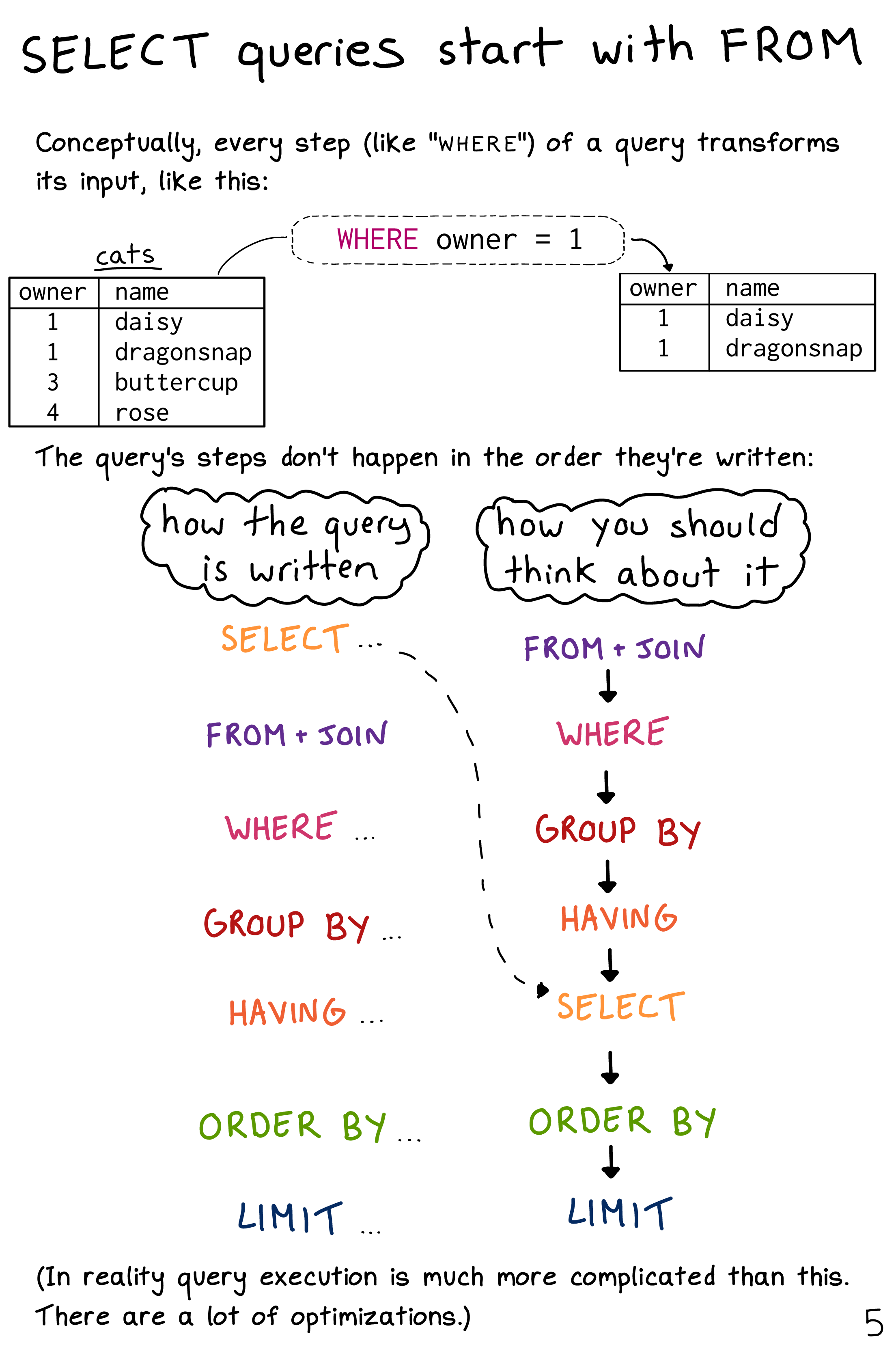

SQL Zine by by Julia Evans

9.2.3 Setup

Let’s get to work.

9.2.4 Packages

pacman::p_load() reduces steps for installing and loading several packages simultaneously.

# pacman 
if (!require("pacman")) install.packages("pacman")

## Loading required package: pacman

# The rest of pkgs 
pacman::p_load(
 tidyverse, # tidyverse packages 
 DBI, # using SQL queries
 RSQLite, # SQLite
 dbplyr, # use database with dplyr 
 glue, # glue to automate workflow 
 nycflights13 # toy data 
)

## Installing package into '/home/jae/R/x86_64-pc-linux-gnu-library/4.2'
## (as 'lib' is unspecified)

## also installing the dependency 'plogr'

## 
## RSQLite installed

9.2.5 NYC flights data

The flight on-time performance data from the Bureau of Transportation Statistics of the U.S. government. The data goes back to 1987, and its size is more than 20 gigabytes. For practice, we only use a small subset of the original data (flight data departing NYC in 2013) provided by RStudio.

From RStudio.

9.2.6 Workflow

Create/connect to a database

Note that the server also can be your laptop (called localhost).
Short answer: To do so, you need interfaces between R and a database. We use RSQLite in this tutorial because it’s easy to set up.
Long answer: The DBI package in R provides a client-side interface that allows dplyr to work with databases. DBI is automatically installed when you install dbplyr. However, you need to install a specific backend engine (a tool for communication between R and a database management system) for the database (e.g., RMariaDB, RPostgres, RSQLite). In this workshop, we use SQLite because it is the easiest to get started with. I love PostgreSQL because it’s open-source and also powerful to do many amazing things (e.g., text mining, geospatial analysis). If you want to build a data warehouse, an analytical platform, consider using Spark (Hadoop).

Copy a table to the database

Option 1: You can create a table and insert rows manually. You also need to define the data schema (the database structure) to do that.
Table
- Collection of rows
- Collection of columns (fields or attributes)
- Each col has a type:
  - String: VARCHAR(20)
  - Integer: INTEGER
  - Floating-point: FLOAT, DOUBLE
  - Date/time: DATE, TIME, DATETIME
- Schema: the structure of the database
  - The table name
  - The names and types of its columns
  - Various optional additional information
    - Constraints
      - Syntax: column datatype constraint
      - Examples: NOT NULL, UNIQUE, INDEX


-- Create table 

CREATE TABLE students (
    id INT AUTO_INCREMENT,
    name VARCHAR(30),
    birth DATE,
    gpa FLOAT,
    grad INT,
    PRIMARY KEY(id));

-- Insert one additional row 

INSERT INTO students(name, birth, gpa, grad)
      VALUES ('Adam', '2000-08-04', 4.0, 2020);

Option 2: Copy a file (object) to a table in a database using copy_to). We take this option as it’s fast, and we would like to focus on querying in this workshop.

Query the table

Main focus

Pull the results of interests (data) using collect()
Disconnect the database

9.2.6.1 Create a database

# Define a backend engine 

drv <- RSQLite::SQLite()

# Create an empty in-memory database 
con <- DBI::dbConnect(drv, 
                      dbname = ":memory:")

# Connect to an existing database 
#con <- DBI::dbConnect(RMariaDB::MariaDB(), 
 # host = "database.rstudio.com",
 # user = "hadley",
 # password = rstudioapi::askForPassword("Database password")
#)

dbListTables(con)

## character(0)

# character(0) = NULL

Note that con is empty at this stage.

9.2.6.2 Copy an object as a table to the database (push)

# Copy objects to the data 
# copy_to() comes from dplyr
copy_to(dest = con, 
        df = flights)

copy_to(dest = con, 
        df = airports)

copy_to(dest = con,
        df = planes)

copy_to(dest = con, 
        df = weather)

# If you need, you can also select which columns you would like to copy:

# copy_to(dest = con, 
#          df = flights, 
#          name = "flights",
#          indexes = list(c("year", "tailnum", "dest")))

# Show two tables in the database 

dbListTables(con)

## [1] "airports"     "flights"      "planes"       "sqlite_stat1" "sqlite_stat4"
## [6] "weather"

# Show the columns/attributes/fields of a table 

dbListFields(con, "flights")

##  [1] "year"           "month"          "day"            "dep_time"      
##  [5] "sched_dep_time" "dep_delay"      "arr_time"       "sched_arr_time"
##  [9] "arr_delay"      "carrier"        "flight"         "tailnum"       
## [13] "origin"         "dest"           "air_time"       "distance"      
## [17] "hour"           "minute"         "time_hour"

dbListFields(con, "weather")

##  [1] "origin"     "year"       "month"      "day"        "hour"      
##  [6] "temp"       "dewp"       "humid"      "wind_dir"   "wind_speed"
## [11] "wind_gust"  "precip"     "pressure"   "visib"      "time_hour"

9.2.6.3 Quick demonstrations:

SELECT desired columns
FROM tables
Select all columns (*) from flights table and show the first ten rows
Note that you can combine SQL and R commands thanks to dbplyr.
Option 1

DBI::dbGetQuery(con, 
                "SELECT * FROM flights;") %>% # SQL
  head(10) # dplyr

##    year month day dep_time sched_dep_time dep_delay arr_time sched_arr_time
## 1  2013     1   1      517            515         2      830            819
## 2  2013     1   1      533            529         4      850            830
## 3  2013     1   1      542            540         2      923            850
## 4  2013     1   1      544            545        -1     1004           1022
## 5  2013     1   1      554            600        -6      812            837
## 6  2013     1   1      554            558        -4      740            728
## 7  2013     1   1      555            600        -5      913            854
## 8  2013     1   1      557            600        -3      709            723
## 9  2013     1   1      557            600        -3      838            846
## 10 2013     1   1      558            600        -2      753            745
##    arr_delay carrier flight tailnum origin dest air_time distance hour minute
## 1         11      UA   1545  N14228    EWR  IAH      227     1400    5     15
## 2         20      UA   1714  N24211    LGA  IAH      227     1416    5     29
## 3         33      AA   1141  N619AA    JFK  MIA      160     1089    5     40
## 4        -18      B6    725  N804JB    JFK  BQN      183     1576    5     45
## 5        -25      DL    461  N668DN    LGA  ATL      116      762    6      0
## 6         12      UA   1696  N39463    EWR  ORD      150      719    5     58
## 7         19      B6    507  N516JB    EWR  FLL      158     1065    6      0
## 8        -14      EV   5708  N829AS    LGA  IAD       53      229    6      0
## 9         -8      B6     79  N593JB    JFK  MCO      140      944    6      0
## 10         8      AA    301  N3ALAA    LGA  ORD      138      733    6      0
##     time_hour
## 1  1357034400
## 2  1357034400
## 3  1357034400
## 4  1357034400
## 5  1357038000
## 6  1357034400
## 7  1357038000
## 8  1357038000
## 9  1357038000
## 10 1357038000

Option 2 (works faster)


SELECT * 
FROM flights 
LIMIT 10

Option 3 (automating workflow)
- When local variables are updated, the SQL query is also automatically updated. This approach is called parameterized query (or prepared statement).

######################## PREPARATION ########################

# Local variables 
tbl <- "flights"
var <- "dep_delay"
num <- 10

# Glue SQL query string 
# Note that to indicate a numeric value, you don't need.

sql_query <- glue_sql("
  SELECT {`var`}
  FROM {`tbl`}
  LIMIT {num} 
  ", .con = con)

######################## EXECUTION ########################

# Run the query 
dbGetQuery(con, sql_query)

##    dep_delay
## 1          2
## 2          4
## 3          2
## 4         -1
## 5         -6
## 6         -4
## 7         -5
## 8         -3
## 9         -3
## 10        -2

Challenge 2 Can you rewrite the above code using LIMIT instead of head(10)?

You may notice that using only SQL code makes querying faster.
Select dep_delay and arr_delay from flights table, show the first ten rows, then turn the result into a tibble.

Challenge 3 Could you remind me how to see the list of attributes of a table? Let’s say you want to see the flights table attributes. How can you do it?

Collect the selected columns and filtered rows

df <- dbGetQuery(con, 
  "SELECT dep_delay, arr_delay FROM flights;") %>%
  head(10) %>%
  collect()

Counting rows
- Count all (*)

dbGetQuery(con, 
          "SELECT COUNT(*) 
           FROM flights;")

##   COUNT(*)
## 1   336776

dbGetQuery(con, 
           "SELECT COUNT(dep_delay)
           FROM flights;")

##   COUNT(dep_delay)
## 1           328521

Count distinct values

dbGetQuery(con, 
           "SELECT COUNT(DISTINCT dep_delay)
           FROM flights;")

##   COUNT(DISTINCT dep_delay)
## 1                       527

9.2.6.4 Tidy-way: dplyr -> SQL

Thanks to the dbplyr package, you can use the dplyr syntax to query SQL.

Note that pipe (%) works.

# tbl select tables
flights <- con %>% tbl("flights")
airports <- con %>% tbl("airports")
planes <- con %>% tbl("planes")
weather <- con %>% tbl("weather")

select = SELECT

flights %>% 
  select(contains("delay"))

## # Source:   SQL [?? x 2]
## # Database: sqlite 3.40.1 [:memory:]
##    dep_delay arr_delay
##        <dbl>     <dbl>
##  1         2        11
##  2         4        20
##  3         2        33
##  4        -1       -18
##  5        -6       -25
##  6        -4        12
##  7        -5        19
##  8        -3       -14
##  9        -3        -8
## 10        -2         8
## # ℹ more rows

Challenge 4 Your turn: write the same code in SQL. Don’t forget to add the connection argument to your SQL code chunk.

mutate = SELECT AS

flights %>%
  select(distance, air_time) %>%  
  mutate(speed = distance / (air_time / 60))

## # Source:   SQL [?? x 3]
## # Database: sqlite 3.40.1 [:memory:]
##    distance air_time speed
##       <dbl>    <dbl> <dbl>
##  1     1400      227  370.
##  2     1416      227  374.
##  3     1089      160  408.
##  4     1576      183  517.
##  5      762      116  394.
##  6      719      150  288.
##  7     1065      158  404.
##  8      229       53  259.
##  9      944      140  405.
## 10      733      138  319.
## # ℹ more rows

Challenge 5 Your turn: write the same code in SQL. ( Hint: mutate(new_var = var 1 * var2 (R) = SELECT var1 * var2 AS near_var (SQL)

filter = WHERE

flights %>% 
  filter(month == 1, day == 1) # filter(month ==1 & day == 1) Both work in the same way.

## # Source:   SQL [?? x 19]
## # Database: sqlite 3.40.1 [:memory:]
##     year month   day dep_time sched_dep_time dep_delay arr_time sched_arr_time
##    <int> <int> <int>    <int>          <int>     <dbl>    <int>          <int>
##  1  2013     1     1      517            515         2      830            819
##  2  2013     1     1      533            529         4      850            830
##  3  2013     1     1      542            540         2      923            850
##  4  2013     1     1      544            545        -1     1004           1022
##  5  2013     1     1      554            600        -6      812            837
##  6  2013     1     1      554            558        -4      740            728
##  7  2013     1     1      555            600        -5      913            854
##  8  2013     1     1      557            600        -3      709            723
##  9  2013     1     1      557            600        -3      838            846
## 10  2013     1     1      558            600        -2      753            745
## # ℹ more rows
## # ℹ 11 more variables: arr_delay <dbl>, carrier <chr>, flight <int>,
## #   tailnum <chr>, origin <chr>, dest <chr>, air_time <dbl>, distance <dbl>,
## #   hour <dbl>, minute <dbl>, time_hour <dbl>

Challenge 6 Your turn: write the same code in SQL (hint: filter(condition1, condition2) = WHERE condition1 and condition2)

Additional tips

Note that R and SQL operators are not exactly alike. R uses != for Not equal to. SQL uses <> or !=. Furthermore, there are some cautions about using NULL (NA; unknown or missing): it should be IS NULL or IS NOT NULL not =NULL or !=NULL (this makes sense because NULL represents an absence of a value).

Another pro-tip is LIKE operator, used in a WHERE statement to find values based on string patterns.

SELECT DISTINCT(origin) -- Distinct values from origin column
FROM flights
WHERE origin LIKE 'J%'; -- Find any origin values that start with "J"

Table 9.1: 1 records
origin
JFK

% is one of the wildcards you can use for string matching. % matches any number of characters. So, J% matches Jae, JFK, Joseph, etc. _ is another useful wildcard that matches exactly one character. So J_ matches only JA, JE, etc. If wildcards are not enough, then you should consider using regular expressions.

arrange = ORDER BY

flights %>% 
  arrange(carrier, desc(arr_delay)) %>%
  show_query()

## <SQL>
## SELECT *
## FROM `flights`
## ORDER BY `carrier`, `arr_delay` DESC

Challenge 7 Your turn: write the same code in SQL. Hint: arrange(var1, desc(var2) (R) = ORDER BY var1, var2 DESC (SQL)

summarise = SELECT AS and group by = GROUP BY

flights %>%
  group_by(month, day) %>%
  summarise(delay = mean(dep_delay))

## `summarise()` has grouped output by "month". You can override using the
## `.groups` argument.

## Warning: Missing values are always removed in SQL aggregation functions.
## Use `na.rm = TRUE` to silence this warning
## This warning is displayed once every 8 hours.

## # Source:   SQL [?? x 3]
## # Database: sqlite 3.40.1 [:memory:]
## # Groups:   month
##    month   day delay
##    <int> <int> <dbl>
##  1     1     1 11.5 
##  2     1     2 13.9 
##  3     1     3 11.0 
##  4     1     4  8.95
##  5     1     5  5.73
##  6     1     6  7.15
##  7     1     7  5.42
##  8     1     8  2.55
##  9     1     9  2.28
## 10     1    10  2.84
## # ℹ more rows

Challenge 8 Your turn: write the same code in SQL (hint: in SQL the order should be SELECT group_var1, group_var2, AVG(old_var) AS new_var -> FROM -> GROUP BY)

If you feel too much challenged, here’s a help.

flights %>%
  group_by(month, day) %>%
  summarise(delay = mean(dep_delay)) %>%
  show_query() # Show the SQL equivalent!

## `summarise()` has grouped output by "month". You can override using the
## `.groups` argument.

## <SQL>
## SELECT `month`, `day`, AVG(`dep_delay`) AS `delay`
## FROM `flights`
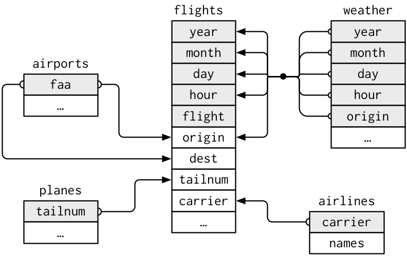
## GROUP BY `month`, `day`

Joins
Using joins is more straightforward in R than it is in SQL.
However, more flexible joins exist in SQL, and they are not available in R.
- Joins involving 3+ tables are not supported.
- Some advanced joins available in SQL are not supported.
- For more information, check out tidyquery to see the latest developments.
SQL command

FROM one table LEFT JOIN another table ON condition = condition (ON in SQL = BY in R)

SELECT *
FROM flights AS f
LEFT JOIN weather AS w 
ON f.year = w.year AND f.month = w.month

Table 9.2: Displaying records 1 - 10
year	month	day	dep_time	sched_dep_time	dep_delay	arr_time	sched_arr_time	arr_delay	carrier	flight	tailnum	origin	dest	air_time	distance	hour	minute	time_hour	origin	year	month	day	hour	temp	dewp	humid	wind_dir	wind_speed	wind_gust	pressure	visib	time_hour
2013	1	1	517	515	2	830	819	11	UA	1545	N14228	EWR	IAH	227	1400	5	15	1357034400	EWR	2013	1	1	1	39.02	26.06	59.37	270	10.35702	NA	1012.0	10	1357020000
2013	1	1	517	515	2	830	819	11	UA	1545	N14228	EWR	IAH	227	1400	5	15	1357034400	EWR	2013	1	1	2	39.02	26.96	61.63	250	8.05546	NA	1012.3	10	1357023600
2013	1	1	517	515	2	830	819	11	UA	1545	N14228	EWR	IAH	227	1400	5	15	1357034400	EWR	2013	1	1	3	39.02	28.04	64.43	240	11.50780	NA	1012.5	10	1357027200
2013	1	1	517	515	2	830	819	11	UA	1545	N14228	EWR	IAH	227	1400	5	15	1357034400	EWR	2013	1	1	4	39.92	28.04	62.21	250	12.65858	NA	1012.2	10	1357030800
2013	1	1	517	515	2	830	819	11	UA	1545	N14228	EWR	IAH	227	1400	5	15	1357034400	EWR	2013	1	1	5	39.02	28.04	64.43	260	12.65858	NA	1011.9	10	1357034400
2013	1	1	517	515	2	830	819	11	UA	1545	N14228	EWR	IAH	227	1400	5	15	1357034400	EWR	2013	1	1	6	37.94	28.04	67.21	240	11.50780	NA	1012.4	10	1357038000
2013	1	1	517	515	2	830	819	11	UA	1545	N14228	EWR	IAH	227	1400	5	15	1357034400	EWR	2013	1	1	7	39.02	28.04	64.43	240	14.96014	NA	1012.2	10	1357041600
2013	1	1	517	515	2	830	819	11	UA	1545	N14228	EWR	IAH	227	1400	5	15	1357034400	EWR	2013	1	1	8	39.92	28.04	62.21	250	10.35702	NA	1012.2	10	1357045200
2013	1	1	517	515	2	830	819	11	UA	1545	N14228	EWR	IAH	227	1400	5	15	1357034400	EWR	2013	1	1	9	39.92	28.04	62.21	260	14.96014	NA	1012.7	10	1357048800
2013	1	1	517	515	2	830	819	11	UA	1545	N14228	EWR	IAH	227	1400	5	15	1357034400	EWR	2013	1	1	10	41.00	28.04	59.65	260	13.80936	NA	1012.4	10	1357052400

Can anyone explain why SQL query using dplyr then translated by show_query() looks more complex than the above? (Hint)

flights %>% 
  left_join(weather, by = c("year", "month")) %>%
  show_query()

## <SQL>
## SELECT
##   `flights`.`year` AS `year`,
##   `flights`.`month` AS `month`,
##   `flights`.`day` AS `day.x`,
##   `dep_time`,
##   `sched_dep_time`,
##   `dep_delay`,
##   `arr_time`,
##   `sched_arr_time`,
##   `arr_delay`,
##   `carrier`,
##   `flight`,
##   `tailnum`,
##   `flights`.`origin` AS `origin.x`,
##   `dest`,
##   `air_time`,
##   `distance`,
##   `flights`.`hour` AS `hour.x`,
##   `minute`,
##   `flights`.`time_hour` AS `time_hour.x`,
##   `weather`.`origin` AS `origin.y`,
##   `weather`.`day` AS `day.y`,
##   `weather`.`hour` AS `hour.y`,
##   `temp`,
##   `dewp`,
##   `humid`,
##   `wind_dir`,
##   `wind_speed`,
##   `wind_gust`,
##   `precip`,
##   `pressure`,
##   `visib`,
##   `weather`.`time_hour` AS `time_hour.y`
## FROM `flights`
## LEFT JOIN `weather`
##   ON (
##     `flights`.`year` = `weather`.`year` AND
##     `flights`.`month` = `weather`.`month`
##   )

9.2.6.5 Collect (pull)

collect() is used to pull the data. Depending on the data size, it may take a long time to run.
The following code won’t work.

Error in UseMethod(“collect”) : no applicable method for ‘collect’ applied to an object of class “c(‘LayerInstance’, ‘Layer’, ‘ggproto’, ‘gg’)”

origin_flights_plot <- flights %>%
  group_by(origin) %>%
  tally() %>%
  ggplot() +
  geom_col(aes(x = origin, y = n)) %>%
  collect()

This works.

df <- flights %>%
  group_by(origin) %>%
  tally() %>%
  collect()

origin_flights_plot <- ggplot(df) +
  geom_col(aes(x = origin, y = n))

origin_flights_plot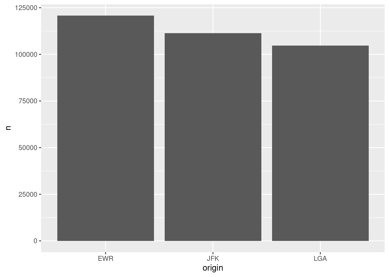

9.2.6.6 Disconnect

DBI::dbDisconnect(con)

9.2.7 Things we didn’t cover

9.2.7.1 Subquery

Subquery = a query nested inside a query

This hypothetical example is inspired by dofactory blog post.

SELECT names  -- Outer query 
FROM consultants
WHERE Id IN (SELECT ConsultingId
                FROM consulting_cases 
                WHERE category = 'r' AND category = 'sql'); -- Subquery

9.2.7.2 Common table expression (WITH clauses)

This is just a hypothetical example inspired by [James LeDoux’s blog post](https://jamesrledoux.com/code/sql-cte-common-table-expressions.

-- cases about R and SQL from dlab-database 
WITH r_sql_consulting_cases AS ( -- The name of the CTE expression 
  -- The CTE query 
  SELECT
    id 
  FROM 
    dlab 
  WHERE
    tags LIKE '%sql%'
  AND
    tags LIKE '%r%'
),
-- count the number of open cases about this consulting category 
-- The outer query 
SELECT status, COUNT(status) AS open_status_count
FROM dlab as d 
INNER JOIN r_sql_consulting_cases as r
  ON d.id = r.id 
WHERE status = 'open';

9.2.8 References

csv2db - for loading large CSV files in to a database
R Studio, Database using R
Ian Cook, “Bridging the Gap between SQL and R” rstudio::conf 2020 slides
- Video recording
Data Carpentry contributors, SQL database and R, Data Carpentry, September 10, 2019.
Introduction to dbplyr
Josh Erickson, SQL in R, STAT 701, University of Michigan
SQL zine by Julia Evans
q - a command-line tool that allows direct execution of SQL-like queries on CSVs/TSVs (and any other tabular text files)