7 Semi-structured data
7.1 Setup
# Install packages
if (!require("pacman")) install.packages("pacman")
## Loading required package: pacman
pacman::p_load(tidyverse, # tidyverse pkgs including purrr
               furrr, # parallel processing
               tictoc, # performance test
               tcltk, # GUI for choosing a dir path
               tidyjson, # tidying JSON files
               XML, # parsing XML
               rvest, # parsing HTML
               jsonlite, # downloading JSON file from web
               glue, # pasting string and objects
               xopen, # opepn URLs in browser
               urltools, # regex and url parsing
               here) # computational reproducibility

## Install the current development version from GitHub
devtools::install_github("jaeyk/tidytweetjson", dependencies = TRUE) ; library(tidytweetjson)
## Skipping install of 'tidytweetjson' from a github remote, the SHA1 (464a7799) has not changed since last install.
## Use `force = TRUE` to force installation7.2 The Big Picture
- Automating the process of turning semi-structured data (input) into structured data (output)
7.3 What is semi-structured data?
Semi-structured data is a form of structured data that does not obey the tabular structure of data models associated with relational databases or other forms of data tables, but nonetheless contains tags or other markers to separate semantic elements and enforce hierarchies of records and fields within the data. Therefore, it is also known as a self-describing structure. - Wikipedia
- Examples: HTML (e.g., websites), XML (e.g., government data), JSON (e.g., social media API)
Below is how JSON (tweet) looks like.
A tree-like structure
Keys and values (key: value)
{ “created_at”: “Thu Apr 06 15:24:15 +0000 2017”, “id_str”: “850006245121695744”, “text”: “1/ Today we019re sharing our vision for the future of the Twitter API platform!://t.co/XweGngmxlP”, “user”: { “id”: 2244994945, “name”: “Twitter Dev”, “screen_name”: “TwitterDev”, “location”: “Internet”, “url”: “https:\/\/dev.twitter.com\/”, “description”: “Your official source for Twitter Platform news, updates & events. Need technical help? Visit https:\/\/twittercommunity.com\/ 3280f #TapIntoTwitter” } }
-
Why should we care about semi-structured data?
- Because this is what the data frontier looks like: # of unstructured data > # of semi-structured data > # of structured data
- There are easy and fast ways to turn semi-structured data into structured data (ideally in a tidy format) using R, Python, and command-line tools. See my own examples (tidyethnicnews and tidytweetjson).
7.4 Workflow
Import/connect to a semi-structured file using
rvest,jsonlite,xml2,pdftools,tidyjson, etc.Define target elements in a single file and extract them
readrpackage providersparse_functions that are useful for vector parsing.stringrpackage for string manipulations (e.g., using regular expressions in a tidy way). Quite useful for parsing PDF files (see this example).rvestpackage for parsing HTML (R equivalent tobeautiful soupin Python)tidyjsonpackage for parsing JSON data
Create a list of files (in this case URLs) to parse
Write a parsing function
Automate parsing process
7.5 HTML/CSS: web scraping
Let’s go back to the example we covered in the earlier chapter of the book.
url_list <- c(
  "https://en.wikipedia.org/wiki/University_of_California,_Berkeley",
  "https://en.wikipedia.org/wiki/Stanford_University",
  "https://en.wikipedia.org/wiki/Carnegie_Mellon_University",
  "https://DLAB"
)- Step 1: Inspection
Examine the Berkeley website so that we could identify a node that indicates the school’s motto. Then, if you’re using Chrome, draw your interest elements, then right click > inspect > copy full xpath.
url <- "https://en.wikipedia.org/wiki/University_of_California,_Berkeley"

download.file(url, destfile = "scraped_page.html", quiet = TRUE)

target <- read_html("scraped_page.html")

# If you want character vector output
target %>%
  html_nodes(xpath = "/html/body/div[3]/div[3]/div[5]/div[1]/table[1]") %>%
  html_text()

# If you want table output
target %>%
  html_nodes(xpath = "/html/body/div[3]/div[3]/div[5]/div[1]/table[1]") %>%
html_table()- Step 2: Write a function
I highly recommend writing your function working slowly by wrapping the function with slowly().
get_table_from_wiki <- function(url){

  download.file(url, destfile = "scraped_page.html", quiet = TRUE)

  target <- read_html("scraped_page.html")

  table <- target %>%
    html_nodes(xpath = "/html/body/div[3]/div[3]/div[5]/div[1]/table[1]") %>%
    html_table()

  return(table)
}- Step 3: Test
get_table_from_wiki(url_list[[2]])- Step 4: Automation
map(url_list, get_table_from_wiki)- Step 5: Error handling
7.6 XML/JSON: government database/social media scraping
7.6.1 Governemnt database (XML)
The following tax return data example comes from the U.S. Internal Revenue Service (IRS) Amazon database. This PDf file shows what the original document looks like.
Workflow
- Get the XML link and parse it
- Go to the root of the XML document
- Identify a specific node you care about
- Get values related to that node
Step1: Get an XML document link
Step 2: Get the page and parse the XML document.
xml_root <- xml_link %>%
  # Get page and parse xml
  xmlTreeParse() %>%
  # Get root
  xmlRoot()

# Data output: list
typeof(xml_root)

# Two elements. Our target is the second one.
summary(xml_root)
Step 3: Get nodes
We grab the mission statement of this org from its tax report (990). // is an XPath syntax that helps to “select nodes in the document from the current node that matches the selection no matter where they are.”
xml_root %>%
  purrr::pluck(2) %>% # Second element (Return Data)
  getNodeSet("//MissionDesc") # Mission statement
Step 4: Get values
7.6.3 Next steps
We will learn how to access and collect data using Twitter and New York Times API. We are going to learn this in two ways: (1) using plug-and-play packages (both using RStudio and the terminal) and (2) getting API data from scratch (httr, jsonlite).
First, sign up for the Twitter developer account before everything else. If you want to know how to sign up for a new Twitter developer account and access Twitter API, see Steinert-Threlkeld’s APSA workshop slides.
7.6.4 rtweet
The rtweet examples come from Chris Bail’s tutorial.
7.6.4.1 Setup
The first thing you need to do is set up.
Assuming that you already signed up for a Twitter developer account
app_name <- "YOUR APP NAME"
consumer_key <- "YOUR CONSUMER KEY"
consumer_secret <- "YOUR CONSUMER SECRET"

rtweet::create_token(app = app_name,
                     consumer_key = consumer_key,
                     consumer_secret = consumer_secret)
7.6.4.2 Search API
Using search API; This API returns a collection of Tweets mentioning a particular query.
# Install and load rtweet
if (!require(pacman)) {install.packages("pacman")}

pacman::p_load(rtweet)
## Warning: package 'rtweet' is not available for this version of R
##
## A version of this package for your version of R might be available elsewhere,
## see the ideas at
## https://cran.r-project.org/doc/manuals/r-patched/R-admin.html#Installing-packages## Warning: 'BiocManager' not available. Could not check Bioconductor.
##
## Please use `install.packages('BiocManager')` and then retry.## Warning in p_install(package, character.only = TRUE, ...):## Warning in library(package, lib.loc = lib.loc, character.only = TRUE,
## logical.return = TRUE, : there is no package called 'rtweet'## Warning in pacman::p_load(rtweet): Failed to install/load:
## rtweet
# The past 6-9 days
rt <- search_tweets(q = "#stopasianhate", n = 1000, include_rts = FALSE)

# The longer term
# search_fullarchive() premium service

head(rt$text)
Can you guess what would be the class type of rt?
class(rt)What would be the number of rows?
nrow(rt)7.6.4.3 Time series analysis
- Time series analysis
pacman::p_load(ggplot2, ggthemes, rtweet)

ts_plot(rt, "3 hours") +
  ggthemes::theme_fivethirtyeight() +
  labs(title = "Frequency of Tweets about StopAsianHate from the Past Day",
       subtitle = "Tweet counts aggregated using three-hour intervals",
source = "Twitter's Search API via rtweet")7.6.5 Hydrating
7.6.5.1 Objectives
- Learning how hydrating works
- Learning how to use Twarc to communicate with Twitter’s API
Review question
What are the main two types of Twitter’s API?
7.6.5.2 Hydrating: An Alternative Way to Collect Historical Twitter Data
You can collect Twitter data using Twitter’s API, or you can hydrate Tweet IDs collected by other researchers. This is an excellent resource to collect historical Twitter data.
Covid-19 Twitter chatter dataset for scientific use by Panacealab
Women’s March Dataset by Littman and Park
Harvard Dataverse has many dehydrated Tweet IDs that could be of interest to social scientists.

7.6.5.3 Twarc: one solution to (almost) all Twitter’s API problems
-
Why Twarc?
A command-line tool and Python library that works for almost every Twitter API-related problem.
-
It’s really well-documented, tested, and maintained.
- Twarc documentation covers basic commands.
- Tward-cloud documentation explains how to collect data from Twitter’s API using Twarc running in Amazon Web Services (AWS).
Twarc was developed as part of the Documenting the Now project, which the Mellon Foundation funded.

There’s no reason to be afraid of using a command-line tool and Python library, even though you primarily use R. It’s easy to embed Python code and shell scripts in R Markdown.
Even though you don’t know how to write Python code or shell scripts, it’s handy to learn how to integrate them into your R workflow.
I assume that you have already installed Python 3.
7.6.5.3.1 Applications
The following examples are created by the University of Virginia library.
7.6.5.3.1.1 Search
Download pre-existing tweets (7-day window) matching certain conditions
In command-line,
>= Create a fileI recommend running the following commands in the terminal because it’s more stable than in R Markdown.

- It is really important to save these tweets into a
jsonlformat;jsonlextension refers to JSON Lines files. This structure is useful for splitting JSON data into smaller chunks if it is too large.
7.6.6 Parsing JSON
7.6.6.1 Objectives
- Learning chunk and pull strategy
- Learning how
tidyjsonworks - Learning how to apply
tidyjsonto tweets
7.6.6.2 Chunk and Pull
7.6.6.2.1 Problem
- What if the size of the Twitter data you downloaded is too big (e.g., >10 GB) to do complex wrangling in R?
7.6.6.2.2 Solution
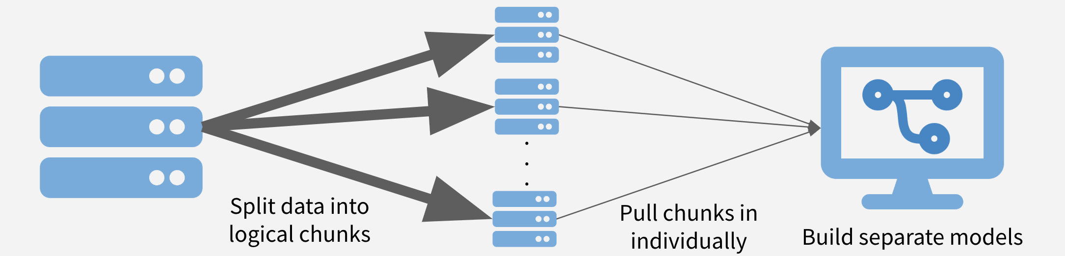
Step1: Split the large JSON file in small chunks.
#Divide the JSON file by 100 lines (tweets)

# Linux and Windows (in Bash)
$ split -100 search.jsonl

# macOS
$ gsplit -100 search.jsonl- After that, you will see several files appear in the directory. Each of these files should have 100 tweets or fewer. All of these file names should start with “x,” as in “xaa.”
Step 2: Apply the parsing function to each chunk and pull all of these chunks together.
# You need to choose a Tweet JSON file
filepath <- file.choose()

# Assign the parsed result to the `df` object
# 11.28 sec elapsed to parse 17,928 tweets
tic()
df <- jsonl_to_df(filepath)
toc()
# Setup
n_cores <- availableCores() - 1

n_cores # This number depends on your computer spec.

plan(multiprocess, # multicore, if supported, otherwise multisession
     workers = n_cores) # the maximum number of workers

# You need to designate a directory path where you saved the list of JSON files.

# 9.385 sec elapsed to parse 17,928 tweets

dirpath <- tcltk::tk_choose.dir()

tic()
df_all <- tidytweetjson::jsonl_to_df_all(dirpath)
toc()
7.6.6.2.3 tidyjson
The tidyjson package helps to use tidyverse framework to JSON data.
- toy example
# JSON collection; nested structure + keys and values
worldbank[1]
## [1] "{\"_id\":{\"$oid\":\"52b213b38594d8a2be17c780\"},\"boardapprovaldate\":\"2013-11-12T00:00:00Z\",\"closingdate\":\"2018-07-07T00:00:00Z\",\"countryshortname\":\"Ethiopia\",\"majorsector_percent\":[{\"Name\":\"Education\",\"Percent\":46},{\"Name\":\"Education\",\"Percent\":26},{\"Name\":\"Public Administration, Law, and Justice\",\"Percent\":16},{\"Name\":\"Education\",\"Percent\":12}],\"project_name\":\"Ethiopia General Education Quality Improvement Project II\",\"regionname\":\"Africa\",\"totalamt\":130000000}"
# Check out keys (objects)
worldbank %>%
  as.tbl_json() %>%
  gather_object() %>%
  filter(document.id == 1)
## # A tbl_json: 8 x 3 tibble with a "JSON" attribute
## ..JSON document.id name
## <chr> <int> <chr>
## 1 "{\"$oid\":\"52b213..." 1 _id
## 2 "\"2013-11-12T00:..." 1 boardapprovaldate
## 3 "\"2018-07-07T00:..." 1 closingdate
## 4 "\"Ethiopia\"" 1 countryshortname
## 5 "[{\"Name\":\"Educa..." 1 majorsector_percent
## 6 "\"Ethiopia Gener..." 1 project_name
## 7 "\"Africa\"" 1 regionname
## 8 "130000000" 1 totalamt
# Get the values associated with the keys
worldbank %>%
  as.tbl_json() %>% # Turn JSON into tbl_json object
  enter_object("project_name") %>% # Enter the objects
  append_values_string() %>% # Append the values
  as_tibble() # To reduce the size of the file
## # A tibble: 500 × 2
## document.id string
## <int> <chr>
## 1 1 Ethiopia General Education Quality Improvement Project II
## 2 2 TN: DTF Social Protection Reforms Support
## 3 3 Tuvalu Aviation Investment Project - Additional Financing
## 4 4 Gov't and Civil Society Organization Partnership
## 5 5 Second Private Sector Competitiveness and Economic Diversificati…
## 6 6 Additional Financing for Cash Transfers for Orphans and Vulnerab…
## 7 7 National Highways Interconnectivity Improvement Project
## 8 8 China Renewable Energy Scale-Up Program Phase II
## 9 9 Rajasthan Road Sector Modernization Project
## 10 10 MA Accountability and Transparency DPL
## # ℹ 490 more rows- The following example draws on my tidytweetjson R package. The package applies
tidyjsonto Tweets.
7.6.6.2.3.1 Individual file
jsonl_to_df <- function(file_path){

# Save file name

file_name <- strsplit(x = file_path,
                     split = "[/]")

file_name <- file_name[[1]][length(file_name[[1]])]

# Import a Tweet JSON file

listed <- read_json(file_path, format = c("jsonl"))

# IDs of the tweets with country codes

ccodes <- listed %>%
  enter_object("place") %>%
  enter_object("country_code") %>%
  append_values_string() %>%
  as_tibble() %>%
  rename("country_code" = "string")

# IDs of the tweets with location

locations <- listed %>%
  enter_object("user") %>%
  enter_object("location") %>%
  append_values_string() %>%
  as_tibble() %>%
  rename(location = "string")

# Extract other key elements from the JSON file

df <- listed %>%
  spread_values(
    id = jnumber("id"),
    created_at = jstring("created_at"),
    full_text = jstring("full_text"),
    retweet_count = jnumber("retweet_count"),
    favorite_count = jnumber("favorite_count"),
    user.followers_count = jnumber("user.followers_count"),
    user.friends_count = jnumber("user.friends_count")
  ) %>%
      as_tibble

message(paste("Parsing", file_name, "done."))

# Full join
outcome <- full_join(ccodes, df) %>% full_join(locations)

# Or you can write this way: outcome <- reduce(list(df, ccodes, locations), full_join)

# Select
outcome %>% select(-c("document.id"))}
7.6.6.2.3.2 Many files
- Set up parallel processing.
n_cores <- availableCores() - 1

n_cores # This number depends on your computer spec.

plan(multiprocess, # multicore, if supported, otherwise multisession
workers = n_cores) # the maximum number of workers- Parsing in parallel.
Review
There are, at least, three ways you can use function + purrr::map().
squared <- function(x){
  x*2
}

# Named function
map(1:3, squared)

# Anonymous function
map(1:3, function(x){ x *2 })

# Using formula; ~ = formula, .x = input
map(1:3,~.x*2)
# Create a list of file paths
filename <- list.files(dir_path,
          pattern = '^x',
          full.names = TRUE)

df <- filename %>%

# Apply jsonl_to_df function to items on the list
future_map(~jsonl_to_df(.)) %>%

# Full join the list of dataframes
reduce(full_join,
       by = c("id",
              "location",
              "country_code",
              "created_at",
              "full_text",
              "retweet_count",
              "favorite_count",
              "user.followers_count",
              "user.friends_count"))

# Output
df
rtweet and twarc
The main difference is using RStudio vs. the terminal.
The difference matters when your data size is large. For example, suppose the size of the Twitter data you downloaded is 10 GB. R/RStudio might have a hard time dealing with this size of data. Then, how can you wrangle this data size in a complex way using R?
7.6.7 Getting API data from scratch
Load packages. For the connection interface, don’t use RCurl, but I strongly recommend using httr. The following code examples draw from my R interface for the New York Times API called rnytapi.
pacman::p_load(httr, jsonlite, purrr, glue)7.6.7.2 Extract data
get_content <- function(term, begin_date, end_date, key, page = 1) {

    message(glue("Scraping page {page}"))

    fromJSON(content(get_request(term, begin_date, end_date, key, page),
                     "text",
                encoding = "UTF-8"),
                simplifyDataFrame = TRUE, flatten = TRUE) %>% as.data.frame()

}
7.6.7.3 Automating iterations
extract_all <- function(term, begin_date, end_date, key) {

    request <- GET("http://api.nytimes.com/svc/search/v2/articlesearch.json",
                   query = list('q' = term,
                                'begin_date' = begin_date,
                                'end_date' = end_date,
                                'api-key' = key))

    max_pages <- (round(content(request)$response$meta$hits[1] / 10) - 1)

    message(glue("The total number of pages is {max_pages}"))

    iter <- 0:max_pages

    arg_list <- list(rep(term, times = length(iter)),
                     rep(begin_date, times = length(iter)),
                     rep(end_date, times = length(iter)),
                     rep(key, times = length(iter)),
                     iter
                     )

    out <- pmap_dfr(arg_list, slowly(get_content,
                                     # 6 seconds sleep is the default requirement.
                                     rate = rate_delay(
                                         pause = 6,
                                         max_times = 4000)))

    return(out)

    }
7.6.2 Social media API (JSON)
7.6.2.1 Objectives
Review question
In the previous session, we learned the difference between semi-structured data and structured data. Can anyone tell us the difference between them?
7.6.2.2 The big picture for digital data collection
Input: semi-structured data
Output: structured data
Process:
Getting target data from a remote server
Parsing the target data your laptop/database
Database (push-parse): Push the large target data to a database, then explore, select, and filter it. If you are interested in using this option, check out my SQL for R Users workshop.
But what exactly is this target data?
When you scrape websites, you mostly deal with HTML (defines a structure of a website), CSS (its style), and JavaScript (its dynamic interactions).
When you access social media data through API, you deal with either XML or JSON (major formats for storing and transporting data; they are light and flexible).
XML and JSON have tree-like (nested; a root and branches) structures and keys and values (or elements and attributes).
If HTML, CSS, and JavaScript are storefronts, then XML and JSON are warehouses.
7.6.2.3 Opportunities and challenges for parsing social media data
This explanation draws on Pablo Barbara’s LSE social media workshop slides.
Basic information
What is an API?: An interface (you can think of it as something akin to a restaurant menu. API parameters are API menu items.)
REST (Representational state transfer) API: static information (e.g., user profiles, list of followers and friends)
Streaming API: dynamic information (e.g, new tweets)
Why should we care?
API is the new data frontier. ProgrammableWeb shows that there are more than 24,046 APIs as of April 1, 2021.
Big and streaming (real-time) data
High-dimensional data (e.g., text, image, video, etc.)
Lots of analytic opportunities (e.g., time-series, network, spatial analysis)
Also, this type of data has many limitations (external validity, algorithmic bias, etc).
Think about taking the API + approach (i.e., API not replacing but augmenting traditional data collection)
How API works
Request (you form a request URL) <-> Response (API responses to your request by sending you data usually in JSON format)
API Statuses
Twitter API is still widely accessible (v2
In January 2021, Twitter introduced the academic Twitter API that allows generous access to Twitter’s historical data for academic researchers
Many R packages exist for the Twitter API: rtweet (REST + streaming), tweetscores (REST), streamR (streaming)
Some notable limitations. If Twitter users don’t share their tweets’ locations (e.g., GPS), you can’t collect them.
The following comments draw on Alexandra Siegel’s talk on “Collecting and Analyzing Social Media Data” given at Montréal Methods Workshops.
Facebook API access has become constrained since the 2016 U.S. election.
Exception: Social Science One.
Also, check out Crowdtangle for collecting public FB page data
Using FB ads is still a popular method, especially among scholars studying developing countries.
YouTube API: generous access + (computer-generated) transcript in many languages
Instragram API: Data from public accounts are available.
Reddit API: Well-annotated text data suitable for machine learning
Upside
Web scraping (Wild Wild West) <> API (Big Gated Garden)
You have legal but limited access to (growing) big data that can be divided into text, image, and video and transformed into cross-sectional (geocodes), longitudinal (timestamps), and historical event data (hashtags). See Zachary C. Steinert-Threlkeld’s 2020 APSA Short Course Generating Event Data From Social Media.
Social media data are also well-organized, managed, and curated data. It’s easy to navigate because XML and JSON have keys and values. If you find keys, you will find observations you look for.
Downside
Rate-limited.
If you want to access more and various data than those available, you need to pay for premium access.